Score-Matching Langevin Dynamics (SMLD)

1 Langevin Dynamics

[!NOTE] How to sample from a distribution The Langevin dynamics for sampling from a known distribution $p(\mathbf{x})$ is an iterative procedure for $t=1,\ldots,T{:}$

$$\mathbf{x}_{t+1}=\mathbf{x}_t+\tau\nabla_\mathbf{x}\log p(\mathbf{x}_t)+\sqrt{2\tau}\mathbf{z},\quad\mathbf{z}\sim\mathcal{N}(0,\mathbf{I}),$$

where $\tau$ is the step size which users can control, and $\mathbf{x}_0$ is white noise.

• Without the noise term, Langevin dynamics is gradient descent.

The intuition is that if we want to sample $\mathbf{x}$ from a distribution, certainly the “optimal” location for $\mathbf{x}$ is where $p(\mathbf{x})$ is maximized (seeing the peak as a representation of a distribution). So the goal of sampling is equivalent to solving the optimization

distribution <=> peak <=> optimal solution

[!IMPORTANT] Langevin dynamics is stochastic gradient descent.

• We do stochastic gradient descent since we want to sample from a distribution, instead of solving the optimization problem.

2 (Stein’s) Score Function

The second component of the Langevin dynamics equation has a formal name known as the Stein’s score function, denoted by

The way to understand the score function is to remember that it is the gradient with respect to the data $\mathbf{x}.$ For any high-dimensional distribution $p(\mathbf{x})$, the gradient will give us vector field $\nabla_\mathbf{x}\log p(\mathbf{x})=\text{a vector field}=\begin{bmatrix}\frac{\partial\log p(\mathbf{x})}{\partial x},&\frac{\partial\log p(\mathbf{x})}{\partial y}\end{bmatrix}^T$

Geometric Interpretations of the Score Function:

• The magnitude of the vectors are the strongest at places where the change of $\log p(\mathbf{x})$ is the biggest. Therefore, in regions where $\log p(\mathbf{x})$ is close to the peak will be mostly very weak gradient.
• The vector field indicates how a data point should travel in the contour map.
• In physics, the score function is equivalent to the “drift”. This name suggests how the diffusion particles should flow to the lowest energy state.

3 Score Matching Techniques

Note that since the distribution is not known, we need some methods to approximate it.

Explicit Score-Matching

Suppose that we are given a dataset $\mathcal{X}=\{\mathbf{x}_1,\ldots,\mathbf{x}_M\}.$ The solution people came up with is to consider the classical kernel density estimation by defining a distribution

where $h$ is just some hyperparameter for the kernel function $K(\cdot)$, and $\mathbf{x}_m$ is the $m$-th sample in the training set.

• The sum of all these individual kernels gives us the overall kernel density estimate $q(\mathbf{x}).$
• The idea is similar to Gaussian Mixture Model.

Since $q(\mathbf{x})$ is an approximation to $p(\mathbf{x})$ which is never accessible, we can learn s$_{\boldsymbol{\theta}}(\mathbf{x})$ based on $q(\mathbf{x}).$ This leads to the following definition of the a loss function which can be used to train a network.

[!IMPORTANT] The explicit score matching loss is

$$J_{\mathrm{ESM}}(\boldsymbol{\theta})\stackrel{\mathrm{def}}{=}\mathbb{E}_{q(\mathbf{x})}\|\mathrm{s}_{\boldsymbol{\theta}}(\mathbf{x})-\nabla_{\mathbf{x}}\log q(\mathbf{x})\|^2$$

By substituting the kernel density estimation, we can show that the loss is

Once we train the network s$_{\boldsymbol{\theta}}$, we can replace it in the Langevin dynamics equation to obtain the recursion:

Issue:

• The kernel density estimation is a fairly poor non-parameter estimation of the true distribution.
• When we have limited number of samples and the samples live in a high dimensional space, the kernel density estimation performance can be poor.

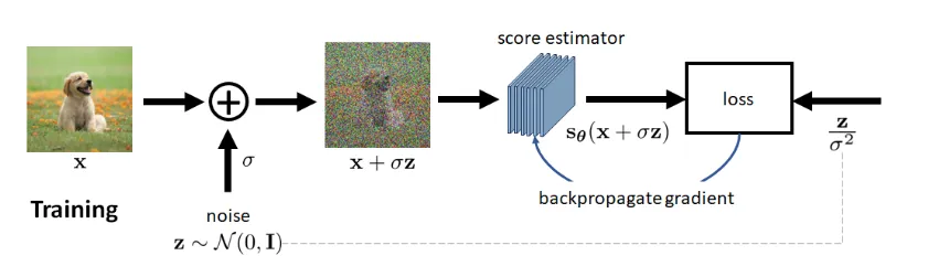
Denoising Score Matching

In DSM, the loss function is defined as follows.

The idea comes from the Denoising Autoencoder approach of using pairs of clean and corrupted examples $(\mathbf{x},\mathbf{x}')$. In the generative model, $\mathbf{x}'$ can be seen as the $\mathbf{x}_{t}$.

The conditional distribution $q(\mathbf{x}|\mathbf{x}^{\prime})$ does not require an approximation. In the special case where $q(\mathbf{x}|\mathbf{x}^{\prime})=\mathcal{N}(\mathbf{x}\mid\mathbf{x}^{\prime},\sigma^2)$, we can let $\mathbf{x}=\mathbf{x}^\prime+\sigma\mathbf{z}.$ This will give us

As a result, the loss function of the denoising score matching becomes

The gradient operation cancels $\mathbf{x}$.

[!IMPORTANT] The Denoising Score Matching has a loss function defined as

$$J_{\mathrm{DSM}}(\boldsymbol{\theta})=\mathbb{E}_{p(\mathbf{x})}\left[\frac12\left\|\mathbf{s}_{\boldsymbol{\theta}}(\mathbf{x}+\sigma\mathbf{z})+\frac{\mathbf{z}}{\sigma^2}\right\|^2\right]$$

• The quantity $\mathbf{x}+\sigma\mathbf{z}$ is effectively adding noise $\sigma\textbf{z}$ to a clean image $\mathbf{x}$.
• The score function $s_{{\boldsymbol{\theta}}}$ is supposed to take this noisy image and predict the noise $\frac {\mathbf{z} }{\sigma ^2}.$
• Predicting noise is equivalent to denoising, because any denoised image plus the predicted noise will give us the noisy observation.

The training step can simply described as follows: You give us a training dataset $\{\mathbf{x}^{(\ell)}\}_{\ell=1}^L$, we train a network $\boldsymbol{\theta}$ with the goal to

The last thing is that why the loss function of DSM makes sense?

[!IMPORTANT] Theorem For up to a constant $C$ which is independent of the variable $\boldsymbol{\theta}$, it holds that

$$J_{\mathrm{DSM}}(\theta)=J_{\mathrm{ESM}}(\theta)+C.$$

The proof is not hard.

For inference, we assume that we have already trained the score estimator s$_{\boldsymbol{\theta}}.$ To generate an image, we perform the following procedure for $t=1,\ldots,T{:}$

Reference

[1] Chan, Stanley H. “Tutorial on Diffusion Models for Imaging and Vision.” arXiv preprint arXiv:2403.18103 (2024).